Introduction
1.1 Background
In video surveillance, video signals from multiple remote locations are displayed on several TV screens which are typically placed together in a control room. In the so-called third generation surveillance systems 3GSS, all the parts of the surveillance systems will be digital and consequently, digital video will be transmitted and processed . Additionally in 3GSS some intelligence has to be introduced to detect relevant events in the video signals in an automatic way. This allows filtering of the irrelevant time segments of the video sequences and the displaying on the TV screen only those segments that require the attention of the surveillance operator. Motion detection is a basic operation in the selection of significant segments of the video signals.
Once motion has been detected, other features can be considered to decide whether a video signal has to be presented to the surveillance operator. If the motion detection is performed after the transmission of the video signals from the cameras to the control room then all the bit streams have to be previously decompressed this can be a very demanding operation especially .If there are many cameras in the surveillance system. For this reason, it is interesting to consider the use of motion detection algorithms operating in the compressed transform domain.
In this thesis we present a motion detection algorithm in the compressed domain with a low computational cost. In the following Section, we assume that video is compressed by using motion JPEG MJPEG, each frame is individually JPEG compressed.
Motion detection from a moving observer has been a very important technique for computer vision applications. Especially in recent years, for autonomous driving systems and driver supporting systems. Vision-based navigation method has received more and more attention world wide.
One of its most important tasks is to detect the moving obstacles like cars, bicycles or even pedestrians while the vehicle itself is running in a high speed. Methods of image differencing with the clear background or between adjacent frames are well used for the motion detection. But when the observer is also moving, which leads to the result of continuously changing background scene in the perspective projection image, it becomes more difficult to detect the real moving objects by differencing methods. To deal with this problem, many approaches have been proposed in recent years.
Previous work in this area has been mainly in two categories: 1) Using the difference of optical flow vectors between background and the moving objects, 2) calibrating the background displacement by using camera’s 3D motion analysis result. Methods developed in calculate the optical flow and estimate the flow vector’s reliability between adjacent frames. The major flow vector, which represents the motion of background, can be used to classify and extract the flow vectors of the real moving objects. However, by reason of its huge calculation cost and its difficulty for determining the accurate flow vectors, it is still unavailable for real applications. To analysis the camera’s 3D motion and calibrate the background is another main method for moving objects detection.
For on-board camera’s motion analysis, many motion-detecting algorithms have been proposed which always expend on the previous recognition results like road lane-marks and horizon disappointing. These Methods show some good performance in accuracy and efficiency because of their detailed analysis of road structure and measured vehicle locomotion, which is, however, computationally expensive and over-depended upon road features like lane-marks, and therefore lead to unsatisfied result when lane mark is covered by other vehicles or not exist at all. Compare with these previous works, a new method of moving objects detection from an on-board camera is presented in this paper. To deal with the background-change problem, our method uses camera’s 3D motion analysis results to calibrate the background scene.
With pure points matching and the introduction of camera’s Focus of Expansion FOE, our method is able to determine camera’s rotation and translation parameters theoretically by using only three pairs of matching points between adjacent frames, which make it faster and more efficient for real-time applications. In section 2, we will interpret the camera’s 3D-motion analysis with the introduction of FOE. Then, the detailed image processing methods for moving objects detection are proposed in section 3 and section 4 which include the corner extraction method and a fast matching algorithm. In section 5 experimental results on real outdoor road image sequence will show the effectiveness and precision of our approach.
1.2 OBJECTIVE
One goal has been to compile an introduction to the motion detection algorithms. There exist a number of studies but complete reference on real time motion detection is not as common .we have collected materials from journals, papers and conferences and proposed an approach that can be best to implement real time motion detection.
Another goal has been to search for algorithms that can be used to implement the most demanding components of an audio encoding and watermarking. A third goal is to evaluate their performance with regard to motion detected. These properties were chosen because they have the greatest impact on the implementation effort.
A final goal has been to design and implement an algorithm. This should be done in high level language or mat lab. The source code should be easy to understand so that it can serve as a reference on the standard for designers that need to implement real time motion detection.
CHAPTER 2
Given a number of sequential video frames from the same source the goal is to detect the motion in the aria observed by the source. When there is no motion all the sequential frames have to be similar up to noise influence. In the case when motion is present there is some difference between the frames. For sure, each low-cost system has some aspect of noise influence. And in case of no motion every two sequential frames will not be the identical.
This why the system must be smart enough to distinguish between noise and real motion. When the system is calibrated and stable enough the character of noise is that every pixel value may be slightly different from that in other frame. And in first approximation it is possible to define some noise per pixel threshold parameter (adaptable for any given state) the meaning of which is how the pixel value (of the same oriented pixel in two sequential frames) might differ but actually the indicating value is the same one. More precisely, if the pixel with coordinates (Xa,Ya) in frame A differs from the pixel with coordinates (Xb,Yb) in frame B less than on TPP (threshold per pixel)
formulae:
if
{abs (Pixel(Xa,Ya)-Pixel(Xb,Yb)) < TPP }
By adapting the TPP value to current system state we can make the system to be noise-stable. By applying this threshold operation to every pixel pair we may assume that all the preprocessed pixel values are noise-free. The element of noise that is not cancelled will be significantly small relative to other part.Ok, if so we have to post-process these values to detect the motion if any. As it was memorized above we have manipulate with different pixels inside two sequential frames to make conclusion about the motion.
Firstly, to make the system sensitive enough we have not to fix the TPP value too big. It mean that keeping the sensitivity of the system high in any two frames there will be some little number (TPP related) of different pixels. And in this case we have not to see them as noise. It is the first of the reasons to define a TPF (threshold per frame) value (adaptable for any given state) the meaning of which is how many pixels at least, inside two sequential frames must differ in order to see them as motion.
The second reason to deal with TPF is to filter (to drop) small motion. For instance, by playing with TPF value we can neutralize motion of the small object (bugs etc.) by still detect the motion of people. And we can write the exact meaning of TPF by formulae:
Lets define NDPPP to be the Number of Different Pre-Processed by TPP Pixels.
So,
there is a motion i.e. NDPPP > TPF.
Both of TPP and TPF values are variable through the UI to get the optimal system sensitivity. Also the TPF value has its visual equivalent and it is used as following. After the pixels pre-processing (by TPP) lets color all static (which do not include motion) pixels by lets say black color and all the dynamic (which indicate the motion) pixels will be left with their original color. This will bring the effect of motion extraction. In the other words, all the static parts of the frames will be black, and only the moving parts will be seen normally. The enabling/disabling of this effect is possible to control through the GUI.
2.2 Camera Driver Routines
The Camera Manager provides routines for acquiring video frames from CCD cameras. Any process can request a video frame from any video source. The system manages a request queue for each source and executes them cyclically.
The Camera Manager routines are:
1. klStartSnap - sends a request for video frame.
2. WaitForSnapEnd - puts the calling process in WAIT state for a number of context switches or till l the end of requested video frame acquisition.
3. klCancelSnap - removes a request for video frame.
For formal definition of Camera Driver routines see the listing of kernel.h file.
CHAPTER 3
NEURAL NETWORKS
3.1 DEFINITION:
A mathematical model to solve engineering problems Group of highly connected neurons to realize compositions of non linear functions.
3.2 TWO TYPES OF NURAL NETWORK
· Feed forward Neural Network
· Back propagation Network
Feed-Forward Neural Network
If we consider the human brain to be the 'ultimate' neural network, then ideally we would like to build a device which imitates the brain's functions. However, because of limits in our tech3nology, we must settle for a much simpler design. The obvious approach is to design a small electronic device which has a transfer function similar to a biological neuron, and then connect each neuron to many other neurons, using RLC networks to imitate the dendrites, axons, and synapses.
This type of electronic model is still rather complex to implement, and we may have difficulty 'teaching' the network to do anything useful. Further constraints are needed to make the design more manageable. First, we change the connectivity between the neurons so that they are in distinct layers, such that each neuron in one layer is connected to every neuron in the next layer. Further, we define that signals flow only in one direction across the network, and we simplify the neuron and synapse design to behave as analog comparators being driven by the other neurons through simple resistors. We now have a feed-forward neural network model that may actually be practical to build and use.
Referring to figures 1 and 2, the network functions as follows: Each neuron receives a signal from the neurons in the previous layer, and each of those signals is multiplied by a separate weight value. The weighted inputs are summed, and passed through a limiting function which scales the output to a fixed range of values. The output of the limiter is then broadcast to all of the neurons in the next layer. So, to use the network to solve a problem, we apply the input values to the inputs of the first layer, allow the signals to propagate through the network, and read the output values.

Figure3.1 Generalized Network. Stimulation is applied to the inputs of the first layer, and signals propagate through the middle (hidden) layer(s) to the output layer. Each link between neurons has a unique weighting value.

Figure 3.2 structure of a neuron
Figure3.2 The Structure of a Neuron. Inputs from one or more previous neurons are individually weighted, then summed. The result is non-linearly scaled between 0 and +1, and the output value is passed on to the neurons in the next layer.
Since the real uniqueness or 'intelligence' of the network exists in the values of the weights between neurons, we need a method of adjusting the weights to solve a particular problem. For this type of network, the most common learning algorithm is called Back Propagation (BP). A BP network learns by example, that is, we must provide a learning set that consists of some input examples and the known-correct output for each case. So, we use these input-output examples to show the network what type of behavior is expected, and the BP algorithm allows the network to adapt.
The BP learning process works in small iterative steps: one of the example cases is applied to the network, and the network produces some output based on the current state of it's synaptic weights (initially, the output will be random). This output is compared to the known-good
CHAPTER 4
SYSTEM DESIGNS
4.1 BLOCK DIAGRAM

4.2 CORRELATION
Correlation is an architecture and learning algorithm for artificial neural networks developed by Scott Fahlman at Carnegie Mellon in 1990. Instead of just adjusting the weights in a network of fixed topology, Cascade-Correlation begins with a minimal network, then automatically trains and adds new hidden units one by one, creating a multi-layer structure.
Once a new hidden unit has been added to the network, its input-side weights are frozen. This unit then becomes a permanent feature-detector in the network, available for producing outputs or for creating other, more complex feature detectors. The Cascade-Correlation architecture has several advantages over existing algorithms: it learns very quickly, the network determines its own size and topology, it retains the structures it has built even if the training set it requires no back propagation of error signals through Network.
4.3 RADIL BASIS FUNCTION
Radial functions are a special class of function. Their characteristic feature is that their response decreases (or increases) monotonically with distance from a central point. The centre, the distance scale, and the precise shape of the radial function are parameters of the model, all fixed if it is linear.

4.4 RADIL BASIS FUNCTION NETWORK
Radial functions are simply a class of functions. In principle, they could be employed in any sort of model (linear or nonlinear) and any sort of network (single-layer or multi-layer). However radial basis function networks (RBF networks) have traditionally been associated with radial functions in a single-layer network such as shown in the figure below.

Position and size. We do use nonlinear optimization but only for the regularization parameter in ridge regression and the optimal subset of basis functions in forward selection. We also avoid the kind of expensive nonlinear gradient descent algorithms (such as the conjugate gradient and variable metric methods ) that are employed in explicitly nonlinear networks. Keeping one foot firmly planted in the world of linear algebra makes analysis easier and computations quicker.

4.6 THE OPTIMAL WEIGHT VECTOR

4.7 PROPSED SYSTEM
This chapter presents the main software design and implementation issues. It starts by describing the general flow chart of the main program that was implemented in MATLAB. It then explains each component of the flow chart with some details. Finally it shows how the graphical user interface GUI was designed.
4.7 .1 Main Program Flow Chart
The main task of the software was to read the still images recorded from the camera and then process these images to detect motions and take necessary actions accordingly. below shows the general flow chart of the main program.
It starts with general initialization of software parameters and objects setup. Then, once the program started the flag value which indicates whether the stop button was pressed or not is checked.
If the stop button was not pressed it start reading the images then process them using one of the two algorithms as the operator was selected. If a motion is detected it starts a series of actions and then it go back to read the next images, otherwise it goes directly to read the next images. Whenever the stop button is pressed the flag value will be set to zero and the program is stopped, memory is cleared and necessary results are recorded. This terminates the program and returns the control for the operator to collect the results.


This process takes approximately 15 seconds to be completed,(depending on the specifications of the PC used) for the serial port it starts by selecting a communication port and reserving the memory addresses for that port, then the PC connect to the device using the communication setting that was mentioned in the previous chapter. The video object is part of the image acquisition process but it should be setup at the start of the program.
4.7.3 Image acquisition

After setup stage the image acquisition starts as shown in figure 4.7.3 above. This process reads images from the PC camera and save them in a format suitable for the motion detection algorithm. There were three possible options from which one is implemented. The first option was by using auto snapshots software that takes images automatically and save them on a hard disk as JPEG format, and then another program reads these images in the same sequence as they were saved.
It was found that the maximum speed that can be attained by this software is one frame per second and this limits the speed of detection. Also, synchronization was required between both image processing and the auto snapshot software’s where next images need to be available on the hard disk before processing them .The second option was to display live video on the screen and then start capturing the images from the screen. This is a faster option from the previous approach but again it faced the problem of synchronization, when the computer monitor goes into a power saving mode where black images are produced all the time during the period of the black screen.
The third option was by using the image acquisition toolbox provided in MATLAB 7.5.1 or higher versions. The image acquisition toolbox is a collection of functions that extend the capability of MATLAB. The toolbox supports a wide range of image acquisition operations, including acquiring images through many types of image acquisition devices, such as frame grabbers and USB PC cameras, also viewing a preview of the live video displayed on monitor and reading the image data into the MATLAB workspace directly.
For this project video input function was used to initialize a video object that connects to the PC camera directly. Then preview function was used to display live video on the monitor. get snapshot function was used to read images from the camera and place them in MATLAB workspace.
The later approach was implemented because it has many advantages over the others. It achieved the fastest capturing speed at a rate of five frames per seconds depending on algorithm complexity and PC processor speed. Furthermore, the problem of synchronization was solved because both capturing and processing of images were done using the same software.
All read images were converted it into a two dimensional monochrome images. This is because equations in other algorithms in the system were designed with such image format.
4.7.4 Motion Detection Algorithm
A motion detection algorithm was applied on the previously read images. There were two approaches to implement motion detection algorithm. The first one was by using the two dimensional cross correlation while the second one was by using the sum of absolute difference algorithm. These are explained in details in the next two sub sections.
4.7.4.1 Motion Detection Using Cross Correlation
First the two images were sub divided into four equal parts each. This was done to increase the sensitivity of calculation where it is easier to notice the difference between part of image rather than a whole one. A two dimensional cross correlation was calculated between each sub image with its corresponding part in the other image.
This process produces four values ranging from -1 to 1 depending on the difference of the two correlated images. Because the goal of this division was to achieve more sensitivity the minimum value of correlation will be used as reference to the threshold. In normal cases, motion can easily be detected when the measured minimum cross correlation value is used to set the threshold. However, detection fails when images contain global variations such as illuminations changes or when camera moves.
Figure above shows a test case that contains consecutive illumination level changes by switching the light on and off. During the time where the lights are on (frames 1-50 and frames 100-145) the correlation value is around 0.998 and when the lights are switched off (frames 51-99 and frames 146-190) the correlation value is around 0.47. If the threshold for detection was fixed around the value of 0.95 it will continuously detect motion during the light off period.

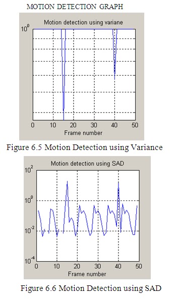
To overcome this problem continuous re-estimation of threshold value was required. This can be done by using an adaptive filter but it is not easy to design. Another solution is to look at the variance of the set of data produced from the cross correlation process, and detect motion from it. This method solved the problem of changing illumination and camera movements.
The variance signal calculated from the same set of images of figure . It can be seen that the need for continuously re-estimate the threshold value is eliminated. Choosing a threshold of 1*10-2 will detect the times when only the lights are switched on and off. This results into a robust motion detection algorithm with high sensitivity of detection.
4.7.4.2 Motion Detection Using Sum of Absolute Difference (SAD)

The above figure shows a test case that contains a large change in the scene being monitored by the camera this was done by moving the camera. During the time before the camera was moved the SAD value was around 1.87 and when the camera was moved the SAD value was around 2.2. If the threshold for detection was fixed around the value less than 2.2 it will continuously detect motion after the camera stop moving.
To overcome this problem the same solution that was applied to the correlation algorithm will be used. The variance value was computed after collecting two SAD values and the result is shown for the same test case in figure 4.7.4.3below.

This approach solve the need for continuously re-estimate the threshold value. Choosing a threshold of 1*10-3 will detect the times when only the camera is moved. This results into a robust motion detection algorithm that can not be affected by illumination change and camera movements.
4.7.5 Actions on Motion Detection
Before explaining series of actions happen when motion is detected it is worth to mention that the values of variance that was calculated .whether it was above or below the threshold will be stored in an array, where it will be used later to produce a plot of frame number Vs the variance value. This plot helps in comparing the variance values against the threshold to be able to choose the optimum threshold value.

whenever the variance value is less than threshold the image will be dropped and only the variance value will be recorded. However when the variance value is greater than threshold sequence of actions is being started .
As the above flow chart show a number of activities happen when motion is detected.
First the serial port is being triggered by a pulse from the PC; this
pulse is used to activate external circuits connected to the PC. Also a log file is being created and then appended with information about the time and date of motion also the frame number in which motion occur is being recorded in the log file. Another process is to display the image that was detected on the monitor. Finally the image that was detected in motion will be converted to a movie frame and will be added to the film structure.
4.7.6 Break and clear Process
After motion detection algorithm applied on the images the program checks if the stop button on GUI was pressed. If it was pressed the flag value will be changed from one to zero and the program will break and terminate the loop then it will return the control to the GUI. Next both serial port object and video object will be cleared. This process is considered as a cleaning stage where the devises connected to the PC through those objects will be released and the memory space will be freed.
4.7.7 Data Record
Finally when the program is terminated a data collection process starts where variable and arrays that contain result of data on the memory will be stored on the hard disk.
This approach was used to separate the real time image processing from results processing. This has the advantage of calling back these data whenever it is required. The variables that are being stored from memory to the hard disk are variance values and the movie structure that contain the entire frames with motion.
At this point the control will be returned to the GUI where the operator can callback the results that where archived while the system was turned on.
Next section will explain the design of the GUI highlighting each button results and callbacks.
4.8 GRAPHICAL USER INTERFACE DESIGN
The GUI was designed to facilitate interactive system operation. GUI can be used to setup the program, launch it, stop it and display results. During setup stage the operator is promoted to choose a motion detection algorithm and select degree of the detection sensitivity.
Whenever the start/stop toggle button is pressed the system will be launched and the selected program will be called to perform the calculations until the start/stop button is pressed again which will terminate the calculation and return control to GUI. Results can be viewed as a log file, movie and plot of frame number vs. variance value. illustrate a flow chart of the steps performed using the GUI.

The complete GUI code is included in the appendix.

.The GUI as shown in figure 4.9 was designed using MATLAB GUI Builder. It consists of two radio buttons, two sliders, two static text box, four push buttons and a toggle button. Sliders and radio buttons were used to prevent entering a wrong value or selection.The radio buttons are being used to choose either SAD algorithm or 2D cross correlation algorithm.
Both algorithms can not be selected at the same time.Sliders are used to select how sensitive the detection is, maximum sensitivity is achieved by moving the slider to the left.
The static text show the instantaneous value of the threshold as read from the sliders. When GUI first launch it will select the optimum value for both algorithms as default vale. Moving to the control panel Start / Stop button is used to launch the program when it is first pushed and to terminate the program when it is pushed again. Figure 4.10 show flow chart of commands executed when this button is pressed.
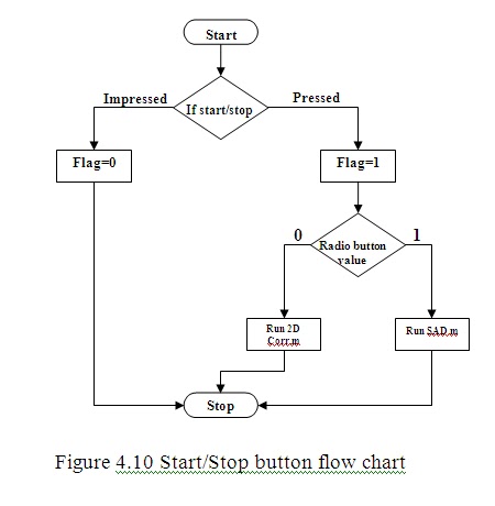
Whenever the Start/Stop button is first pushed it will set the value of the flag to 1 then it will check the value of the radio buttons to determine which main program to launch. A log file that contains information about time and date of motions with frame number is being opened when the log file icon is pushed.
The program is being closed and MATLAB is shutdown when the exit button is pushed. Whenever the show movie icon is pushed, MATLAB will load the film structure that was created before from the hard disk then it will convert the structure into a movie and display it on the screen at a rate of 5 frames per seconds. Finally the movie created will be compressed using the Indeo3 compression technique and will be saved on the hard disk under the name [film.avi]. Figure 4.11below show the commands executed when this icon is pushed.

CHAPTER 5
CODING
Function varargout = guidemo(varargin)
% GUIDEMO M-file for guidemo.fig
% GUIDEMO, by itself, creates a new GUIDEMO or raises the existing
% singleton*.
% H = GUIDEMO returns the handle to a new GUIDEMO or the handle to
% the existing singleton*.
% GUIDEMO('CALLBACK',hObject,eventData,handles,...) calls the local
% function named CALLBACK in GUIDEMO.M with the given input
% GUIDEMO('Property','Value',...) creates a new GUIDEMO or raises the
% existing singleton*. Starting from the left, property value pairs are
% applied to the GUI before guidemo_OpeningFunction gets called. An
% unrecognized property name or invalid value makes property application
% stop. All inputs are passed to guidemo_OpeningFcn via varargin.
% *See GUI Options on GUIDE's Tools menu. Choose "GUI allows only
% instance to run (singleton)".
% See also: GUIDE, GUIDATA, GUIHANDLES
% Edit the above text to modify the response to help guidemo
% Last Modified by GUIDE v2.5 05-Mar-2006 13:40:49
% Begin initialization code - DO NOT EDIT
gui_Singleton = 1;
gui_State = struct('gui_Name', mfilename, ...
'gui_Singleton', gui_Singleton, ...
'gui_OpeningFcn', @guidemo_OpeningFcn, ...
'gui_OutputFcn', @guidemo_OutputFcn, ...
'gui_LayoutFcn', [] , ...
'gui_Callback', []);
if nargin & isstr(varargin{1})
gui_State.gui_Callback = str2func(varargin{1});
end
if nargout
[varargout{1:nargout}] = gui_mainfcn(gui_State, varargin{:});
else
gui_mainfcn(gui_State, varargin{:});
end
% End initialization code - DO NOT EDIT
% --- Executes just before guidemo is made visible.
function guidemo_OpeningFcn(hObject, eventdata, handles, varargin)
% This function has no output args, see OutputFcn.
% hObject handle to figure
% eventdata reserved - to be defined in a future version of MATLAB
% handles structure with handles and user data (see GUIDATA)
% varargin command line arguments to guidemo (see VARARGIN)
% Choose default command line output for guidemo
handles.output = hObject;
% Update handles structure
guidata(hObject, handles);
% UIWAIT makes guidemo wait for user response (see UIRESUME)
% uiwait(handles.figure1);
% --- Outputs from this function are returned to the command line.
function varargout = guidemo_OutputFcn(hObject, eventdata, handles)
% varargout cell array for returning output args (see VARARGOUT);
% hObject handle to figure
% eventdata reserved - to be defined in a future version of MATLAB
% handles structure with handles and user data (see GUIDATA)
% Get default command line output from handles structure
varargout{1} = handles.output;
% --- Executes on button press in Browse.
function Browse_Callback(hObject, eventdata, handles)
% hObject handle to Browse (see GCBO)
% eventdata reserved - to be defined in a future version of MATLAB
% handles structure with handles and user data (see GUIDATA)
[filename, pathname] = uigetfile('*.avi', 'Pick an video');
if isequal(filename,0) | isequal(pathname,0)
warndlg('File is not selected');
else
handles.filename=filename;
% Update handles structure
guidata(hObject, handles);
end
% --- Executes on button press in GetFrames.
function GetFrames_Callback(hObject, eventdata, handles)
% hObject handle to GetFrames (see GCBO)
% eventdata reserved - to be defined in a future version of MATLAB
% handles structure with handles and user data (see GUIDATA)
b='.bmp';
file=handles.filename;
% file='video.AVI';
frm=aviread(file);
Fileinfo = aviinfo(file);
Frmcnt =length(frm);
% Frmcnt = Fileinfo.NumFrames ;
h = waitbar(0,'Please wait...');
for i = 1:Frmcnt
A1 = aviread(file,i);
B1 = frame2im(A1);
Filename=strcat(num2str(i),b);
imwrite(B1,Filename);
waitbar(i/Frmcnt,h)
end
close(h)
warndlg('Frame seperation process completed');
% --- Executes on button press in Correlation.
function Correlation_Callback(hObject, eventdata, handles)
% hObject handle to Correlation (see GCBO)
% eventdata reserved - to be defined in a future version of MATLAB
% handles structure with handles and user data (see GUIDATA)
tic;
a=1;
file=handles.filename;
% file='video.AVI';
frm=aviread(file);
Fileinfo = aviinfo(file);
Frmcnt =length(frm);
delete log.txt
NAME='.bmp';
aaa=get(handles.slider,'Value')
% aaa=0.8
threshold=aaa;
%start a for loop that equal the number of images usually infinity
Frmcnt=Frmcnt-1;
for l = 1:Frmcnt
a=a+1;
first =num2str(l);
kk=l+1;
first1 =num2str(kk);
filename=strcat(first,NAME);
filename1=strcat(first1,NAME);
a1=imread(filename);
b1=imread(filename1);
v=imresize(a1,[288 352]);
w=imresize(b1,[288 352]);
x= rgb2gray (v);
%convert image to gray scale
%dividing a 240 by 320 into 4 pictures
x1=x(1:144,1:176);
x2=x(1:144,177:352);
x3=x(145:288,177:352);
x4=x(145:288,1:176);
y= rgb2gray(w);
%convert image to gray scale
%dividing a 240 by 320 into 4 pictures
y1=y(1:144,1:176);
y2=y(1:144,177:352);
y3=y(145:288,177:352);
y4=y(145:288,1:176);
%mesure of 2 dimensions cross correlation for each picture
z= corr2(x,y);
z1= corr2(x1,y1);
z2= corr2(x2,y2);
z3= corr2(x3,y3);
z4= corr2(x4,y4);
%put values of correlation into arrays
h(a) = z;
h1(a)=z1;
h2(a)=z2;
h3(a)=z3;
h4(a)=z4;
%measure the minimum value for correlation
hh=[z1,z2,z3,z4];
var_value=min(hh);
var_value1(l)=var_value;
save var_value1 var_value1
if (var_value < threshold)
%check if value of variance greater than threshold
fid = fopen('log.txt','a');
%write date,time and frame number into log file log.txt
time=datestr(now)
fprintf(fid,'MOTION WAS DETECTED AT %-100.20s\n',time);
fprintf(fid,'In Frame Number %-110.5d\n',a);
fclose(fid);
else
end %end of if statment
%end of if statment (flag)
toc
end %end of for loop
warndlg('PROCESS COMPLETED');
% --- Executes on button press in SAD.
function SAD_Callback(hObject, eventdata, handles)
% hObject handle to SAD (see GCBO)
% eventdata reserved - to be defined in a future version of MATLAB
% handles structure with handles and user data (see GUIDATA)
clc;
clear;
tic;
a=1;
delete log_sad.txt
NAME='.bmp';
threshold=1;
%start a for loop that equal the number of images usually infinity
for l = 1:49
a=a+1;
first =num2str(l);
kk=l+1;
first1 =num2str(kk);
filename=strcat(first,NAME);
filename1=strcat(first1,NAME);
a1=imread(filename);
b1=imread(filename1);
v=imresize(a1,[288 352]);
w=imresize(b1,[288 352]);
x= rgb2gray (v); %convert image to gray scale
y= rgb2gray(w);
z = imabsdiff(x,y); %get absolute diffrence between both images
zz= sum(z,1); %calculate SAD
zzz= sum(zz)/ 101376; %scale the value of SAD by dividing by number of pixels
h = zzz; %put values of SAD in array h
%calculate variance value
var_value=h;
% var_values(a)=var_value; %put values of variance in array var_value
var_value2(l)=var_value;
save var_value2 var_value2
if (var_value > threshold) %check if value of variance greater than threshold
fid = fopen('log_sad.txt','a'); %write date,time and frame number into log file log.txt
time=datestr(now)
fprintf(fid,'MOTION WAS DETECTED AT %-100.20s\n',time);
fprintf(fid,'In Frame Number %-110.5d\n',a);
fclose(fid);
else
end %end of if statment
%end of if statment (flag)
toc
end %end of for loop
warndlg('PROCESS COMPLETED');
% --- Executes on button press in play_movie.
function play_movie_Callback(hObject, eventdata, handles)
% hObject handle to play_movie (see GCBO)
% eventdata reserved - to be defined in a future version of MATLAB
% handles structure with handles and user data (see GUIDATA)
[filename, pathname] = uigetfile('*.avi', 'Pick an video');
if isequal(filename,0) | isequal(pathname,0)
warndlg('File is not selected');
else
a=aviread(filename);
axes(handles.one);
movie(a);
end
% --- Executes on button press in clear.
function clear_Callback(hObject, eventdata, handles)
% hObject handle to clear (see GCBO)
% eventdata reserved - to be defined in a future version of MATLAB
% handles structure with handles and user data (see GUIDATA)
a=ones(256,256);
axes(handles.one);
imshow(a);
delete *.txt;
warndlg('Files cleared succesfully');
% --- Executes on button press in Exit.
function Exit_Callback(hObject, eventdata, handles)
% hObject handle to Exit (see GCBO)
% eventdata reserved - to be defined in a future version of MATLAB
% handles structure with handles and user data (see GUIDATA)
exit;
% --- Executes on button press in Pass_code.
function Pass_code_Callback(hObject, eventdata, handles)
% hObject handle to Pass_code (see GCBO)
% eventdata reserved - to be defined in a future version of MATLAB
% handles structure with handles and user data (see GUIDATA)
% --- Executes on button press in View_LOGFILE.
function View_LOGFILE_Callback(hObject, eventdata, handles)
% hObject handle to View_LOGFILE (see GCBO)
% eventdata reserved - to be defined in a future version of MATLAB
% handles structure with handles and user data (see GUIDATA)
open 'log.txt';
% --- Executes on button press in Plot_Graph_Corr.
function Plot_Graph_Corr_Callback(hObject, eventdata, handles)
% hObject handle to Plot_Graph_Corr (see GCBO)
% eventdata reserved - to be defined in a future version of MATLAB
% handles structure with handles and user data (see GUIDATA)
cla;
load var_value1;
semilogy(var_value1);
grid on;
xlabel('Frame number');
ylabel('VARIANCE VALUE');
title('Motion detection using variane');
% --- Executes on button press in Analysis.
function Analysis_Callback(hObject, eventdata, handles)
% hObject handle to Analysis (see GCBO)
% eventdata reserved - to be defined in a future version of MATLAB
% handles structure with handles and user data (see GUIDATA)
ana
% --- Executes on button press in View_Log_SAD.
function View_Log_SAD_Callback(hObject, eventdata, handles)
% hObject handle to View_Log_SAD (see GCBO)
% eventdata reserved - to be defined in a future version of MATLAB
% handles structure with handles and user data (see GUIDATA)
open 'log_sad.txt';
% --- Executes on button press in Plot_Graph_SAD.
function Plot_Graph_SAD_Callback(hObject, eventdata, handles)
% hObject handle to Plot_Graph_SAD (see GCBO)
% eventdata reserved - to be defined in a future version of MATLAB
% handles structure with handles and user data (see GUIDATA)
cla;
load var_value2;
axes(handles.one);% figure;
semilogy(var_value2);
grid on;
xlabel('Frame number');
ylabel('VARIANCE VALUE');
title('Motion detection using SAD');
% --- Executes during object creation, after setting all properties.
function slider_CreateFcn(hObject, eventdata, handles)
% hObject handle to slider (see GCBO)
% eventdata reserved - to be defined in a future version of MATLAB
% handles empty - handles not created until after all CreateFcns called
% Hint: slider controls usually have a light gray background, change
% 'usewhitebg' to 0 to use default. See ISPC and COMPUTER.
usewhitebg = 1;
if usewhitebg
set(hObject,'BackgroundColor',[.9 .9 .9]);
else
set(hObject,'BackgroundColor',get(0,'defaultUicontrolBackgroundColor'));
end
% --- Executes on slider movement.
function slider_Callback(hObject, eventdata, handles)
% hObject handle to slider (see GCBO)
% eventdata reserved - to be defined in a future version of MATLAB
% handles structure with handles and user data (see GUIDATA)
% Hints: get(hObject,'Value') returns position of slider
% get(hObject,'Min') and get(hObject,'Max') to determine range of slider
a=get(hObject,'Value')
% t2 = get(hObject,'Value')
a=num2str(a);
%
set(handles.t1,'String',a);
% --- Executes during object creation, after setting all properties.
function t1_CreateFcn(hObject, eventdata, handles)
% hObject handle to t1 (see GCBO)
% eventdata reserved - to be defined in a future version of MATLAB
% handles empty - handles not created until after all CreateFcns called
% Hint: edit controls usually have a white background on Windows.
% See ISPC and COMPUTER.
if ispc
set(hObject,'BackgroundColor','white');
else
set(hObject,'BackgroundColor',get(0,'defaultUicontrolBackgroundColor'));
end
function t1_Callback(hObject, eventdata, handles)
% hObject handle to t1 (see GCBO)
% eventdata reserved - to be defined in a future version of MATLAB
% handles structure with handles and user data (see GUIDATA)
% Hints: get(hObject,'String') returns contents of t1 as text
% str2double(get(hObject,'String')) returns contents of t1 as a double
| |
RESULTS AND DISCUSSION
We have tested our algorithm in different video sequences and, in general, after the calibration period, the algorithm allows motion to be detected correctly. In the following we show results obtained in detecting motion in a video sequence (384 x 288 pixels, 12.5 frames/s) of 71 frames long. Initially (from frame 1 to frame 32) there is no motion in the scene. From frame 33 to frame 6 1, somebody comes in, goes through and comes out of the scene. Finally, from frame 62 to frame 71, no motion occurs. From frame 1 to 10, the scene is conveniently illuminated, then the illumination intensity decreases suddenly in frame 11 and the scene remains low illuminated until frame 23. In frame 24 good illumination suddenly increases and the scene remains well illuminated until frame 46, in which illumination suddenly decreases and remains at this level until the end of the video sequence.


Figure 6.4 Log file or SAD

CHAPTER 7
CONCLUSION
We have presented an algorithm to detect motion in video sequences. It has a very low computational cost. After a period of calibration in which the threshold value is set, the algorithm is able to detect moving blocks in every frame by counting sign changes in the quadrants.
The number of moving blocks per frame allows determination of the periods of time with motion. It seems to be simulation in stimulant processor provides accuracy rather than real time motion detection using m files. So here we concluded that real time motion detection can be best implemented by our propose approach based on correlation network and sum and absolute difference.
CHAPTER-8
FEATURE ENHANCEMENT
This paper describes 3D motion detection system. Five special designed neural networks are introduced. They are the correlation network, the rough motion detection network, the edge enhancement network, the background remover and the normalization network.
This project provides the object image clearly when it is in motion. The motion detection image is captured within 9-10 seconds. The same function can be implemented in moving cameras as for an easy surveillance. And the images captured within 2-4 seconds with the precise algorithm using a multiple input. (More crowded images). Since there were only two objects detected, it took only 8 seconds, for the processing of all three stages.
CHAPTER -9
REFERENCES
1) 'Special issue on third generation surveillance systems', froc. IEEE, 2008, JAIN, R., KASTURI, R., and SCHUNCK, B.G.:
2) Y. Song, A perceptual approach to human motion detection and labeling. PhD thesis,California Institute of Technology, 2003.
3) 'Motion video sensor in the compressed domain'. SCS Euromedia Conf., Valencia, Spain, 2001
4) N. Howe, M. Leventon, and W. Freeman, “Bayesian reconstruction of 3D human motion from single-camera video,” Tech. Rep. TR-99-37, Mitsubishi Electric Research Lab, 1999.
5) L. Goncalves, E. D. Bernardo, E. Ursella, and P. Perona, “Monocular tracking of the human arm in 3D,” in Proc. 5th Int. Conf. Computer Vision, Cambridge, Mass, pp. 764– 770, 1995.
6) S. Wachter and H.-H. Nagel, “Tracking persons in monocular image sequences,” Computer Vision and Image Understanding, vol. 74, pp. 174–192, 1999.
7) D. Gavrila, “The visual analysis of human movement: A survey,” Computer Vision and Image Understanding, vol. 73, pp. 82–98, 1999.


2 comments:
Would this be able to track smaller objects like animals or does it just work on larger objects like people/cars?
Will you share your code with me...I would like to try it. Thanks
Post a Comment