Xray Imaging using Pseudo coloring Matlab

ABSTRACT

Samples with the same color or appearance in the visible region of the electromagnetic spectrum, which are therefore indistinguishable to the Human eye, can have different properties in other parts of the spectrum. Basically, the reflectance or transmittance spectra of these samples are expected to be similar in the visible region, but can differ in other regions.

In this work we present a system, which uses the information included in five spectral bands of the near-infrared region of the spectrum (NIR, 800-1000 nm) in order to discriminate samples with the same appearance in the visible. The system, based on the images registered by a CCD camera, permits us to obtain falsely colored images of the samples using a color space representation which associates the camera responses of each spectral band of the near-infrared to a color channel of a calibrated device, in our case a CRT monitor.

We write a simple program to convert gray level image to pseudo color images. By altering the conditions and values used in the program, we can create a more perfect pseudo color image.

Pseudo coloring:

Pseudo color image processing shall be an important tool in digital processing of breast images. Pseudo coloring comprises of assigning colors to gray values based on a specific criterion. The term Pseudo color or false color is used to differentiate the process of assigning colors to monochrome images from the process associated with true color images. The first and foremost use of pseudo color is for human visualization and Interpretation of gray scale events in an image or sequent of images. The Principal cause of using color is the fact that humans can discern thousands if color shades and intensities, compared to only two dozen or shades of gray.

Introduction

Achieving higher detection rates of threat objects during airport luggage inspection is a pressing and sought-after goal for airport and airplane security personnel. Luggage inspection is an essential process for airports and airplane security because of the presence of large crowds (customers and personnel) and a history of terrorists’ patterns in airports and on airplanes. On the other hand, luggage inspection has always been a challenge due to the complexities present in knowing the content of each individual bag. The drastic growth in various technologies has also led to an increase in the level of sophistication and methods of device concealment by terrorists. The problems are compounded by considerations of a screener constantly gazing at a screen and seeing almost the same type of objects over and over again.

The purpose of this research is to enhance the x-ray image obtained form a luggage inspection to provide better differentiation of the scene components. The idea is to assist the operator in identifying items requiring hand inspection, by focusing his/her attention on regions whose image characteristics indicate the potential for containing a threat object. This capability will increase the efficiency of the operation of luggage inspection by decreasing the time required to perform inspection and reducing the probability of errors due to fatigue. By automating or semi-automating the process of inspection at carry-on luggage stations, an increase in speed and customer convenience will accrue. However, this increase in speed should not come at the expense of an increase in the rate of false alarms. This is why it is very important to consider speed of inspection, accuracy of detection of threat, and lower false alarm rates all simultaneously when designing an efficient system or implementing a new algorithm. This can be achieved in various ways, one of which is by using effective color-coding schemes.

The advantages of using color over grayscale display are to be determined in this study. Color is very commonly used in various applications including visualization, graphical user interfaces, imaging, internet browsers and many other computer related applications. The fundamental question that may arise is “why use color?” simple but ultimate reason is “people prefer it”. Color shapes the perception, interpretation and memory of everything visualized. “Color can be a powerful tool to improve the usefulness of an information display in a wide variety of areas if used properly. Conversely, the inappropriate use of color can seriously reduce the functionality of a display system.” Color is a major component in GUI’s. Appropriate color use can aid user memory and facilitate the formation of effective mental models. As noted above, the effective use of color can be a powerful tool. However, ineffective use of color can degrade an application's performance and lessen user satisfaction.

In order to create an expert system with effective colors the following questions have to be answered.

• How effective colors can be chosen, which provide good differentiation between different objects?

• How many colors can be displayed?

• Which color space should be used?

• What factors determine target element color relative to the non-target elements?

In an attempt to answer these questions, an extensive color study is carried out. The focus is directed towards physiological and psychological factors, which govern color perception. These factors are studied carefully and various guidelines are derived for developing an expert system.

Color is used in a qualitative rather than a quantitative fashion, that is, to show that one item is different form another, rather than to display the relationship of degree. Consider the X-ray image shown in Figure 1, the image does reveal the hidden threat but when the coloring scheme is analyzed,

the following questions arise.

• Is that color scheme good enough for an operator?

• Is that background good enough for visualization?

• Is the number of colors used good enough for visualization?

Previous work has addressed the issues of choosing color for certain type of data visualization and user interfaces. These works are analyzed and discussed in this paper. Although it is impossible to develop a complete set of guidelines for the effective use of color, some broad principles based on the previous work and guidelines for modeling is established and an expert system is modeled. Based on the results efficient color-coding schemes were designed and implemented. The effectiveness of using color-coding schemes over grayscale representation is established by conducting an online survey. The results are tabulated and statistical analyses are carried out.

1.1 History:

Airport luggage inspection has always been a challenge because of

(1) the complexity naturally present in knowing the content of each individual bag,

(2) the constant increase in the level of sophistication and methods of device

concealment by terrorists, and

(3) the decrease in screeners’ alertness when constantly gazing at a screen and

seeing almost the same type of objects over and over again.

Traditionally, potential threats are thought of as metallic guns and knives; that is, object made from high-density materials. After September 11, 2001, the Transportation Security Administration (TSA) made public a lot of newly prohibited threat items—among others, plastic, glass, and wooden sharp objects that can be used as knives. These objects are made of low-density materials. This increase in the types of potential threat objects significantly compounded luggage inspection problems. A number of techniques based on x-rays, gamma rays, electromagnetic field, and millimeter waves have been employed for detecting weapons and explosives.

X-ray based techniques are the most common means used in airports for luggage inspection for the following reasons:

(1) X-ray technology can help provide information on the objects’ density and their effective atomic number (The “effective atomic number” is the estimate of a hypothetical single element that will give the same x-ray attenuation as the substance being evaluated);

(2) X-ray technology has been developed for over a century;

(3) X-ray technology is safer to human beings and luggage contents than other radiations such as nuclear magnetic resonance;

(4) X-ray physics is well understood; and

(5) X-rays are less expensive and easy to operate.

Different x-ray techniques are used in airports for the inspection of luggage. Among the most popular methods are conventional transmission imaging, dual energy x-ray imaging, scatter imaging and 3D imaging. In this thesis, the focus will be on conventional single energy and dual energy x-ray luggage detection systems. Conventional x-ray systems are effective in detecting objects of metallic composition (knives and guns), while low-density weapons could easily go unchecked. Objects such as metallic guns and knives, which are characterized by high-density responses in x-ray images, are also easily spotted by screeners.

However, objects like plastic, glass, and wooden sharp items are characterized by very faint, low-density responses in x-ray projections and are very hard to distinguish by screeners. Commercial dual energy x-ray systems are used to identify materials in luggage by comparing two images of the luggage obtained at two different x-ray energy levels and estimating the atomic number of the materials. However, the real density of objects is poorly known and only an estimate of atomic number can be generated, i.e. effective atomic number. As a result of these limitations, the false alarm rate of dual energy x-ray luggage detection systems reaches to roughly 30%.

Introduction to Mat lab

What is Matlab?

Matlab (short for MATrix LABoratory) is a language for technical computing, developed by the ‘The Mathworks’, Inc. It provides a single platform for computation, visualization, programming and software development. All problems and solutions in Matlab are expressed in notation used in linear algebra and essentially involve operations using matrices and vectors.

As part of the undergraduate Electrical Engineering program, you will be using Matlab to solve problems in

Circuits
Communication systems
Digital signal processing
Control systems
Probability and statistics

In addition, you can use Matlab to build Graphical User Interfaces (GUIs) so that you can develop user-friendly custom software.

The Matlab software environment has a core module (called Matlab) and associated with that are a set of "Toolboxes" that perform specialized computations.

Part I. BASICS

I. Assigning Values to Variables, Vectors and Matrices

Use the equality symbol, e.g. A=3
Variables are case sensitive: temperature is not the same as Temperature
To check values, just type the variable name
There are special constants already available, e.g. pi, Inf
For complex numbers, either use 3+2i or 3+2j
Vectors and matrices are enclosed with square brackets:

a) Elements of rows are separated by commas: A=[1,2,3]

b) Elements of columns are separated by semicolons: B=[1;2;3]

c) Matrices can be seen as columns of row vectors, C=[1,2,3;4,5,6]

Alternatively, use spaces to separate row elements and return keys for column elements:

B = [ 1 2 3

4 5 6

1 0 1 ]

To get size information,

a) size(A) yields [# rows, # cols]

b) size(A,1) yields # rows

c) size(A,2) yields # cols

d) length(v) yields # elements in vector v

Some shortcuts are available:

a) A = 1:0.1:2 yields a row vector [1, 1.1, 1.2, … , 1.9, 2]

b) diag([1,2,3]) yields a diagonal matrix [1,0,0 ; 0,2,0 ; 0,0,3]

c) diag([1,2,3],1) yields a matrix [ 0,1,0,0 ; 0,0,2,0 ; 0,0,0,3 ; 0,0,0,0 ]

d) eye(4) yields an identity matrix of size 4x4

e) zeros(3) yields a matrix of zeros of size 3x3

f) zeros(size(A)) yields a matrix of zeros having the same size as A

g) ones(3), ones(2,5), ones(size(A)) works the same as zeros() except it produces a matrix of ones

h) rand(m,n) matrix of uniformly distributed random numbers of size m by n

i) randn(m,n) matrix of normally distributed random numbers of size m by n

j) linspace(a,b,n) creates a vector of n elements linearly spaced from a to b

k) logspace(a,b,n) creates a vector of n elements logarithmically spaced from 10a to 10b

Vectors and matrices can be appended to build larger matrices, e.g. E=[A,B;C,D]
To disable the echoing results you could include a semicolon after each command line.
To check existing list, you could type who or who’s
To extract elements:

a) A(1,2) gives the element at row 1 and column 2

b) A(3,:) gives the third row of A

c) A(:,4) gives the fourth column of A

d) A([3,2],[2,1]) extracts rows 3 and 2, and columns 2 and 1

To remove rows and columns:

a) A(2,:)=[] removes the 2nd row

b) A(:,1)=[] removes the 1st column

Reshaping and vectorization

a) A(:) yields a vectorized column [a11 ; a21 ; …;an1 ; …; a1n; …;ann]

b) reshape(A,m,n) yields a matrix of size m by n by building it column-wise

II. Matrix Operations and other operations

matrix operations

addition C=A+B
multiplication C=A*B
determinant c=det(A)
inverse inv(A) or A^(-1)
right division C=B/A (same as C=B*inv(A) )
left division C=A\B (same as C= inv(A)*B )
transpose C=A.' ( Note: C=A' is conjugatetranspose)
exponentiation B=A^3
matrix exponentiation B=expm(A)
rank R=rank(A)
eigenvalue/eigenvectors [Eigenvals,Eigenvecs] = eig(A)
characeristic polynomial p = poly(A)
12 Kronecker product C=kron(A,B)
trace t=trace(A)
pseudo-inverse M = pinv(A)

polynomials

roots of polynomial R = roots([ 1, 4, 2] ) ( = roots of s2+4s+2=0 )
polynomial, given roots p=poly([r1,r2])
polynomial multiplication p=conv( [1, 4, 2],[-2, 3] ) ( = (s2 + 4s + 2)(-2s+3) )

column-wise operation

column-wise sum s=sum([1,2,3;4,5,6]) ( = [ 5,7,9] )
column-wise product p=prod([1,2,3;4,5,6]) ( = [ 4, 10, 18] )

sorting

sort cols in ascending order V = sort(A) if A = [ 5, 3 ] then V= [ 1, 3 ] [ 1, 4 ] [5, 4 ]
sorting and getting indices [V,K] = sort(A)

Element wise operation: precede operator by a dot, e.g. A.*B, A./B, A.^2

III. Plotting

2D plots

plot(x,y) uses default

plot(x,y,x,z) combines plot of y vs x and z vs x

plot(x,y,'-',x,z,'--') specifies how each plot is drawn: solid line for x-y and dashed for x-z

Labeling

xlabel('Time (sec)') labeling the x-axis

ylabel('Temperature') labels the y-axis

title('Case 1') puts title on top of plot

text(1.2, 3.0, 'Case 1') puts text on specified location

gtext('Case 2') text is place with the aid of the mouse (or use the menu bar in the figure window)

You can use a limited version of TeX formatting for

a) greek letters and other symbols (see TeX manual) ' \alpha \nabla T ' yields a text : 

b) subscript and superscripts: 'T_{surround}^{a+b}' yields a text : Tsurround

a+b

Axis settings

axis([0,10,-1,1]) specifies x-range as 0 to 10, and y-range as -1 to 1

axis('square') makes the plot square

axis returns to automatic axis mode

hold freezes the previous plot

3D plots

[x,y]=meshgrid(-10:0.5:10, -2:0.2:2) initializes x and y matrices ( for the following try z=sin(x/2).*sin(y) )

mesh(x,y,z) mesh plot

surf(x,y,z) surface plot

surfl(x,y,z) surface plots with lighting

shading interp smoothens shading scheme as interpolated

colormap(gray) changes coloring scheme to gray scale

brighten(-0.5) darkens picture ( if >0 then it brightens)

view([10,60]) changes view to azimuth=10o and elevation=60o

IV. Printing

print sends plot to printer

print h:\sample1.ps saves the plot as a file

print -deps h:\sample2.eps specifies format (or you can use the menu in the figure window)

V. Workspaces

clear erases all variables

clear a, B, Temperature erases only specified variables

diary h:\case1.dry saves all terminal activity and saves in file

case1.dry

save h:\assign1.mat saves workspace

save h:\assign1.mat a, B saves only specified variables

save h:\assign1.mat a, B –ascii saves in ascii format

load h:\assign1.mat loads workspace

load h:\data1.any loads from a file and creates a matrix named data1 ( or you can use menu items for importing data and changing paths)

VI. Some helpful tips

help grabs help information from functions or script files cursor up and down keys scrolls through previous commands

VI. Multidimensional Arrays

a) Creating arrays of higher dimensions

- Method 1: set using assignments

Given: A=[1,2; 3,4]

Then type: A(:,:,2)= [11, 22; 33, 44]

- Method 2: using cat function

Given: A=[1,2 ; 3,4]

B = [11 , 22; 33, 44]

Then type: C=cat(3,A,B)

- Method 3: using “ones”, “zeros” and “repmat”

b) Dimensions and Reshaping arrays

ndims(A) gets the number of dimensions of A

size(A) gets the size of each dimension of A

reshape(A,[m,n,p]) reshapes A into a multidimensional array of size [m,n,p] by first collecting all elements of A in a column and then distributing according to the specified size.

c) Permuting arrays

permute(A,[2,1,3]) changes the dimension indexing, (where 1,2,3 are the this is essentially like the transpose, except dimensions, not sizes) it applies on any dimension.

VII. Structures

Features/Motivation:

- helps encapsulate and organize information of different types

- uses text fields, instead of numeric fields

- can be collected as arrays

- can have subfields

- most commands require the options to come from structures

- most commands can output to structures

a) Creating Structures

Method 1: Use period to create fields and subfields

student.IDNumber=1234;

student.Name='Hank Hill';

Method 2: Use the struct command

student=struct('IDNumber',1234,...

'Name','Hank Hill');

For building structure arrays, just start numbering

student(2)=struct('IDNumber',5678,...

'Name','Robert Plant');

b) Extracting Information: just type the structure name including the fields

student(2)

student(2).Name

c) Removing fields

student = rmfield( student , 'IDNumber' )

VIII. Cell Arrays

Features/Motivation

- Cell arrays are similar to structures except you use numeric indices.

- Instead of matrices, cell arrays can have different types of elements

a) Creation:

Use assignments with “curly brackets”

A = { [1,2;3,4], ‘Testing’; {[1,2] ;3}} , 3+5i }

b) Extracting information:

A{1,1} should yield the element in {1,1}

A{2,1}{1,1} assuming element {2,1} is a cell, then extracts the {1,1} element

c) Translating to structures and vice versa:

C=cell2struct(A(:),...

{'matrix','name','vector','cell'})

D=struct2cell(C); this converts structure C to cell array arranged in a column

E=reshape(D,2,2); this will reshape cell array D

IX. M-files

M-file scripts:

To solve complicated problems, you don't have to use MATLAB interactively. Instead, you can type all commands in an ASCII file named with .m extension. It is called a script file or an M-file. For instance, you can type the while-loop example in a file called example.m using any text editor or using the Open M-file item in the File menu. In MATLAB, use cd path to change to the directory including example.m, then just type example, and the commands in this file will be executed. You can also use pwd in MATLAB to see your present working directory.

When you choose a filename for an M-file, avoid the variable names you may use and the names of MATLAB built-in functions. You can use the command who to see all variables you have used in a session, and use help to see if a name is a built-in function.

Features/Motivation

- using the Matlab editor or any text editor such as notepad

- to write a user-define function that could take different inputs and yields different outputs

- collect subfunctions together for better organization of files

- several Matlab functions need user-supplied functions in forms of m-files.

a) Example 1. ( simple function )

function y = example1(A,x,b)

% y = example1(A,x,b)

% ===================

% solves for y=Ax+b

% @ Michigan Technological University

y = A*x + b ;

b) Example 2. ( different inputs and outputs)

function [y,norm] = example2(A,x,b)

% [y,norm] = example2(A,x,b)

% ==========================

% obtains

% a) y = Ax+b

% b) or y = Ax if b not included

% c) norm = sqrt( y' * y )

y = A*x;

if nargin==3

y = y + b;

end

if nargout == 2, % if norm is required

norm=y'*y;

end

c) Example 3. ( includes sub functions)

function y norms = example3(Y)

% ynorms = example3(Y)

% ====================

% obtains ynorms = [ ynorm1, ..., ynormn ]

% where ynormi= xnorm( y(:,i) )

% xnorm(x) = sqrt(x'*x)

nycols = size(Y,2);

ynorms =[];

for i = 1:nycols

ycol = Y(:,i);

ynorms=[y norms , newnorm(y cool)];

end

function x norm = new norm (x);

xnorm = sqrt(x'*x);

Image processing

Introduction

· Operations that modify the intensity (gray level values) of individual pixels are known as Point Operations.

· If the operation is independent of the location of the pixel, then it is called as a Homogeneous Point Operation.

· A LUT is a table that implements a mapping between current and target pixel values.

· Typically used for:

1. Pseudo Colouring

2. Compensate non-linearity's in sensor elements

A Simple Operation : Transpose

Gray Level Histograms:

nGray Level Histogram shows the distribution of intensities, regardless of their coordinate positions.

nIs a graph which shows the frequency of occurrence in each of the different intensity levels within the image.

nShape of the Gary Level Histogram describes several properties of the image such as overall brightness, contrast etc.

Image Statistics – Histogram:

Gray level histogram:

These problems in an image can be rectified based on techniques that affect the gray level histograms.

Pseudo coloring:

3. Factors

Color is a particular sensation created in the brain, caused when light radiation of a certain wavelength reaches our eyes. This definition is built up from two parts, which are quite different. The first is of a psychological nature. This portion deals with the way the sensation of color is processed by the mind. The second one is merely the eye’s detection of physical radiant energy. Therefore, color is in fact a psychophysical phenomenon, inter-relating both psychological and physical processes.

3.1 Physiological Factors

Color is determined by an interaction among three photopigments; the perceived color is a mixture of the relative responses of the red, green, and blue photopigments, in much the same way as a television camera creates color. Given a dramatic imbalance among the percentages of cells containing red (approximately 64%), green (approximately 32%), and blue (approximately 2%) photopigments, it is clear that the perception of color is both highly specialized and physiologically biased.

Color results from the interaction of light with the nervous system. There are several components that affect color perception, including the eye lens, the retina, and a color processing unit along the optic nerve. These areas are discussed in the following sections.

3.1.1 Lens

The function of the lens is to focus the incoming light on the retina, which contains the photoreceptors. Different wavelengths of light have different focal lengths. Therefore, for pure hues, the lens must change its shape so that the light is focused correctly. For a given lens curvature, longer wavelengths have a longer focal length, i.e., red is the longest focal length and blue is the shortest. To have an image focused on the retina, the lens curvature must change with wavelength with red light requiring the greatest curvature and blue light the least curvature. This means that if pure blue and pure red hues are intermixed, the lens is constantly changing shape and the eye becomes tired.

A related effect is called chromostereopsis, here pure colors located at the same distance from the eye appear to be at different distances, e.g. reds appear closer and blues more distant. Sometimes pure blues focus in front of the retina and so appear unfocused. At night, a deep blue sign may appear fuzzy while other colors appear sharp. The lens also absorbs light about twice as much in the blue region as in the red region. As people age the lens yellows, which means it absorbs more in the shorter wavelengths. Therefore, the result is that people are more sensitive to longer wavelengths (yellows and oranges) than they are to shorter wavelengths (cyan to blue) and these increases with age. The fluid between the lens and the retina also absorb light and this effect increases as people age, so the older people get the less sensitive they are to light in general (the apparent brightness level decreases) and especially the sensitivity to blue decreases.

3.1.2 Retina

The retina contains the photoreceptors that absorb photons and transmit chemical signals to the brain. There are two types: rods, which are night-vision receptors and have no color dependency, and cones, which have color sensitivity and require a higher level of light intensity than the rods.

Figure 5. Spectral sensitivities of the three classes of photoreceptors in the retina,

As shown in Figure2, there are three types of photo-pigments in the cones; "blue" with a maximum sensitivity at 430 nm, "green" with a maximum sensitivity at 530 nm, and "red" at 560 nm. (This wavelength actually corresponds to yellow). Light at a single wavelength will partially activate all three types of cones, e.g. at a wavelength of 470 nm, blue is strongest plus some red and green components. The percentage of cones is not equal but is as follows: blue (4%), green (32%), and red (64%). In addition, the cones are differentially distributed in the retina. The center of the retina has a dense concentration of cones but no rods while the periphery has many rods but few cones. The color distribution is also asymmetrical. The center of the retina is primarily green cones, surrounded by red-yellow cones, with the blue cones being mainly on the periphery. The center of the retina has no blue cones. Objects are seen by edge detection, where an edge can be created by a difference in color or brightness or both. Edges formed by color differences alone, with no brightness differences, appear fuzzy and unfocused, so changes in brightness should be added to get sharp edges.

Photoreceptors adjust their sensitivity to the overall light level, e.g. going into or out of a dark room require some adjustment time. There is also a required minimum intensity level for the photoreceptors to respond. This minimum varies with wavelength with the highest sensitivity in the center of the spectrum. Therefore, blues and reds must have a higher intensity than greens or yellows in order to be perceived.

3.1.3 Brain

From the retina, the optic nerve (actually a collection of nerves) connects to the brain but before it reaches the brain, there is a color-processing unit, called the lateral geniculate body.

This recombines the RGB color information into three new channels as follows:

R-G gives red or green color perception

R+G gives the perception of brightness and yields yellow (Y)

Y-B gives yellow or blue color perception

Thus, blue plays no part in brightness so that colors differing only in amount of blue don't produce sharp edges. Also, note that since blue and yellow and red & green are linked together it is impossible to experience combinations such as reddish green or bluish yellow.

3.1.4 Color blindness

About nine percent of the population has some kind of color perception problem. The most common is red-green deficiency, which can arise from a deficiency of either the red or the green photo-pigments. These people have difficulty distinguishing any color that is dependent upon the red : green ratio.

3.1.5 General guidelines based on physiology

These are some of the guidelines drawn from Murch [5] principles based on physiology.

Avoid the simultaneous display of highly saturated, spectrally extreme colors. This causes the lens to rapidly change shape and thus tires the eyes. Desaturate the colors or else use colors that are close together in the spectrum.
Pure blue should be avoided for text, thin lines, and small shapes. Since there are no blue cones in the center of the retina, these are difficult to see. But blue makes an excellent background color, e.g. for a computer display it tends to blur the raster lines.
Avoid adjacent colors that differ only in the amount of blue. Since blue does not contribute to brightness, this creates fuzzy edges.
Older operators need higher brightness levels to distinguish colors.
Colors change in appearance as the ambient light level changes.
The magnitude of a detectable change in color varies across the spectrum.
It is difficult to focus upon edges created by color alone.
Avoid red and green in the periphery of large displays.
Opponent colors go well together.
For color-deficient observers, avoid single color distinctions.

Color selection guidelines based on human color vision

Avoid adjacent areas of strong blue and strong red in a display to prevent unwanted depth effects (colors appearing to lie in different planes).
Never use the blue channel alone for fine detail such as text or graphics. Do not use, for example, blue text on a black background or yellow text on a white background.
Areas of strong color and high contrast can produce afterimages when the viewer looks away from the screen, resulting in visual stress from prolonged viewing.
Do not use hue alone to encode information in applications where serious consequences might ensue if a color-deficient user were to make an incorrect selection.

3.2 Psychological Factors

As well understood as the physiology of color is, this factor provides little explanation for our opinions of color and color combinations. At the very least, opinions of color are learned and highly associative. For example, as children, we often had a “favorite color” and we liked everything: clothes, toys, books that matched our preference. Over time, we learned a variety of color schemes and in most cases, our tastes become more refined. But even as adults, we are influenced by fashion, and may still associate our more sophisticated sense of color with increasingly more sophisticated emotions, desires, or impressions. For example, even a cursory examination of changes in interior design from the 1950s to the present reveals a dramatic evolution of what was considered warm or even comfortable color combinations. A lively debate still rages about the psychology of color, and various claims are made for using color in the environment to stimulate, calm, or enhance the performance of individuals.

Color psychology is a vast field in which color-constancy, simultaneous contrast, the effects of various backgrounds on color perceptions, and so on, are examined, and competing explanations are debated.

Colors tend to look darker and smaller against white, and lighter and larger against black, as shown in Figure 4. The apparent changes in size arise, at least in part, from flare in the eye’s optics, which causes light from the bright areas to be scattered into the neighboring dark areas.

Figure 5. Colors look darker and smaller against a white background and lighter and larger against black.

Colored surroundings can cause a colored region to appear tinged with the complementary hue of the surround, an effect known as chromatic induction. This relativity of color can be used to enrich a display, and it has many applications in art and design. Nevertheless, it can also cause the viewer to see colors differently from the way the designer intended them. Chromatic induction can make the same colors look different (Figure 5a) or different colors look the same (Figure 5b). With recognizable objects, judgments about the color are made in the present image according to memories that have been amassed from our experience of looking at similar objects. Studies have revealed a discrepancy between memory colors and the colors of actual objects and significant changes in saturation may occur in some cases.

Figure 6. (a) Simultaneous contrast can make the same colors look different.

(b) Simultaneous contrast can make different colors look the same

Two objects of the same color may appear markedly different in color depending on background color. The ineffective use of colors can cause vibrations and shadows; images that distract the user and may cause eye strain.

The proper use of color communicates facts and ideas more quickly and aesthetically to the user. Color can also help develop workable, efficient mental models if simplicity, consistency, clarity, and language of color are followed [2,4].

3.2.1 Simplicity

There is an inherent simplicity in color, which should be used when developing the design. The four physiologically primary colors are red, green, yellow and blue. These colors are easy to learn and remember. A color scheme should be simple; according to Miller the magic number for short term memory is seven plus or minus two (7 ± 2). When using color in interfaces the number of colors should not exceed five plus or minus two (5 ± 2). Limit the palette per screen to what the eye can actually keep track of at one glance, usually about six colors depending on the complexity of the screen design. The background color affects the effectiveness of the other colors. Pick an effective background color and use only about five colors.

The number of colors on the screen should be limited accordingly. If the user is overwhelmed or confused by too many colors vying for his attention, he is unlikely to develop an effective mental model.

3.2.2 Consistency

Consistency is vital when assigning meanings to colors. The intuitive ordering of colors can help establish intuitive consistency in the design. The spectral and perceptual order red, green, yellow, blue can guide the order of the concepts attached to colors. Red is first in the spectral order and focuses in the foreground, green and yellow focus in the middle, while blue focuses in the background. Color can be used to encode or chunk information items. This helps increase the number of items a user can retain in short-term memory. Avoid changing the meaning of colors for different screens in the interface.

There are physiological aspects that hinder consistency in the use of color. Various shades of the same color should be avoided for different concepts and ideas. This is especially true for the blues. Different shades of blue are very difficult to distinguish and may not be recognized as different by the user. If the concept is different, use a different color. Avoid using colors that appear differently due to variation in background color. These may be perceived as different colors by the user and meaning will be lost.

3.2.3 Clarity

Clarity is also an important guideline for using color. Experiments have shown that the search time for finding an item is decreased if the color of the item is known ahead of time, and if the color only applies to that item. Standardized interface colors should be established and used across the development. The clear, concise use of color can help users find items more quickly and efficiently.

3.2.4 Color selection guidelines based on color perception

Guidelines drawn from principles based on psychology are:

Surrounding colors, field size, and viewing conditions can all change the appearance of colors.
Where accurate visual judgment of a color is necessary, the surrounding should be a neutral mid-gray to avoid unwanted perceptual color changes.
Color can described more meaningfully in terms of the perceptual dimensions of lightness, hue, and colorfulness than in terms of device signals.

4. Selection of Color Model

Several color models are organized into two basic divisions. These divisions are perceptually based models and display based models. As the names suggest, the first is organized similar to the way color is perceived, and the second is based on the characteristics of a display device.

4.1 Perceptually based models

HSV (hue, saturation, and value) and HLS (hue, light, and saturation) are two perceptually based models Figure 7(a, b). Hue is the spectral wavelength composition of color that produces the colors seen by the human eye, such as orange, blue, etc. Saturation (chroma) is the relative purity of the color on a scale from gray to the most vibrant tone of the particular color. Value is the strength or darkness of the color. Lightness, also referred to as brightness, refers to the amount of light energy creating the color. The HSV system is based on the Munsell color system used by designers, artists and manufacturers. HLS was developed at Tektronix in 1978 to provide a more perceptual model than the display-based model Tektronix was using at the time.

4.2 Display based models

The most common display-based models are RGB and YIQ/YUV. The RGB color model is composed of the primary colors Red, Green, and Blue. This system defines the color model that is used in most color CRT monitors and color raster graphics. They are considered the "additive primaries" since the colors are added together to produce the desired color. The RGB model uses the cartesian coordinate system as shown in Figure 8(a). Notice the diagonal from (0, 0, 0) black to (1, 1, 1) white, which represents the gray-scale. YIQ/YUV is used for TV broadcasting.

Figure 7. (a) HLS – (Hue, Lightness, Saturation) developed by Gerald Murch at Tektronix, late 1970s, perhaps a “truer” representation than HSV, compared to RGB cube rotated

(b) HSV - Hue, Saturation, Value;

Figure 8. (a) RGB color space

(b) CMYK color space

The International Commission on Illumination is a worldwide organization that developed the first version of the spectrally measured model known as CIE in 1931. CIE is a precise spectral measurement used to pinpoint colors and remove color ambiguity. The CIE model is physically based; therefore, it does not fit well into either the perceptually based or the display-based categories. All colors displayed on a computer must be translated into the RGB color space. Unfortunately, there is not a one-to-one mapping from the perceptually based models to the display-based. This fact can explain some of the difficulties encountered when recreating the right color for an interface screen. The exact shade is not always obtained. The CIE model allows translations from HSV to RGB.

Limitations of RGB model

The RGB color coordinates are device-dependent, so they won’t in general reproduce the same color from one display to another.
The model isn’t perceptually uniform, meaning that one unit of coordinate distance doesn’t correspond to the same perceived color difference in all regions of the color space.
It’s difficult to relate this model to color appearance because its basis is device signals (drive voltages) and not display luminance values.
The RGB cube doesn’t easily lend itself to perceptual tasks because there is no correspondence to the human dimensions of color perception (as described in the previous section).

Limitations of HSV and HLS:

Although these models provide better approximations to the perceptual dimensions of color than the simple RGB model, they still have serious limitations:

They remain device-dependent because these models are defined directly in terms of the display RGB drive signals.
None of the three axes is perceptually uniform, which makes it difficult to predict how adjusting the controls by a given amount will affect a color.
The three axes are perceptually dependent. Therefore, a change in one component usually affects the appearance of the others.

4.3 General guidelines for color space

Guidelines drawn for usage of color space are:

RGB display signals are device-dependent, and the color they produce will generally differ from one display to another.
When colors are to be rendered accurately, a calibrated display and gamma correction software should be used for best results.
Use perceptual color models based on CIE uniform color spaces instead of the simplistic color models based on device-dependent RGB signals should be used.
The RGB space does not correspond to the human color perception and does not separate the luminance component from the chromatic ones. Thus, HSV space is preferred. HSV space is naturally intuitive and approximately, perceptual uniform. It is characterized by the coordinates of hue, saturation and value (brightness) based upon human color perception organization.

5. Implementation

The task is to implement various color-coding schemes to x-ray images yielding visually more attractive and pleasing images to the screener which will assist the operator in threat identification and reduce the time required for inspection. Color-coding a grayscale image implies mapping all the gray values in the original image to a meaningful color. This is also referred to as pseudo coloring or false coloring since the color information is added to the original image. This helps in enhancing different pixel ranges in the image and highlights or brings out the region of interest in the image. Color-coding can be achieved in various ways.

Methods discussed here are:

1. Mapping using mathematical functions

2. Applying look up tables

3. Thresholding

5.1 Mapping using mathematical functions

In this method, mathematical functions are utilized to perform the required transformation from gray scale to color. This is performed in the RGB color space. The idea underlying this approach is to perform three independent transformations of the gray level of any input pixel. The three results are combined together as red, green and blue channel to produce a color-coded image. The output images color content is modulated by the nature of the transformation functions.

Figure 9. Functional block diagram for color-coding using transformation

Figure 9 explains the approach, using a functional block diagram. Channel1, channel 2 and channel3 correspond to red, green and blue channel respectively. Trigonometric functions were used as the transformation function. Sine and cosine functions are used and in each channel and the gray values are transformed. By varying the phase and frequency of cycles different color-coding is achieved.

Figure 10 shows the transformation used for implementing sine map.

Figure 10. Transformation used to create sine map

The range of value in each channel should be between 0 and 1. Since the input image is a 16-bit image, the value is normalized by dividing it with 65535. If the value produced by transformation in each channel are equal (channel1=channel2=channel3) then the output image will be monochrome. Figure 11 (a) and (b) shows the input original image and its corresponding output after applying sine transformation.

(a) (b)

Figure 11. (a) Original grayscale image (b) Output image obtained after applying sine

transformation clearly showing the threats (dark red and purple glass knives)

Similar method is implemented using a cosine function. Figure 12 shows the transformation involved.

Figure 12. Transformation used to create cosine map

Again, the phase and the frequency can be varied to achieve different color combinations. After a series of trails, the efficient values are found. At these values, the lower pixels (dark) from original grayscale image are enhanced and easily visible.

Figure 11 (a) and (b) shows the input original image and its corresponding output after applying cosine transformation.

Figure 13. (a) Original grayscale image (b) Output image obtained after applying cosine transformation clearly showing the threats (dark red and purple glass knives)

As mentioned earlier, the various parameters can be changed to obtain different color coding schemes. In order to make this task easier a graphical user interface was created where the parameters can be comfortably adjusted to produce corresponding coding schemes.

The GUI is setup in such a way that by changing the different parameters different color map will be generated. The Figure 14 below shows the input X-ray image colored by two different schemes.

Figure 14. Graphical user interface for generating color-coding schemes

The GUI has adjustable provisions for setting phase and setting the frequency of cycles.

It shows the input x-ray image in two formats original grayscale and negative of that image. The transformation is also plotted in an x-y scale, which helps us to study how the function varies. Using this GUI, different images from the x-ray image database are tested. The combination of values for which the threat objects were best detected was noted.

This color scheme is implemented in RGB space and the major draw back is that the colors used are not controlled and the output image is based on the type of transformation used.

5.2 Applying look up tables (LUT)

A look up table is a m-by-3 matrix of real numbers between 0.0 and 1.0. Each row is an RGB vector that defines one color. The kth row of the colormap defines the k-th color, where map (k,:) = [r(k) g(k) b(k)]) specifies the intensity of red, green, and blue. These tables can be created using some mathematical functions. Figure 15 shows a pseudo code for creating such LUT.

Figure 15. Pseudo-code for creating a look up table

This color map (LUT) is applied to the original grayscale image to obtain pseudo colored output image. Figure 16 shows the input grayscale image and the corresponding colored output image obtained by applying a rainbow map.

Figure 16. Input x-ray image followed by the output obtained by applying rainbow LUT

The grayscale image has a threat (gun), which is enhanced in the output image. The corresponding LUT is shown in figure 17a. The values in the look up tables are plotted to R, G and B respectively and shown in figure 17b.

Figure 17. (a) Sample look up table and (b) the values from the table plotted into R, G and B respectively Several other color maps are produced by this method. Only the most prominent color map (rainbow) is listed here.

5.3 Thresholding

The application of image threshold techniques for the selective visualization of certain gray-level brackets, leads to isolated and enhanced threat representations. This method is developed based on the results derived from the color study discussed earlier. The basic procedure is as follows:

(1). The thresholds are set

(2). The number of colors to be used is defined

(3). The hues to be used are defined

(4). In the HSV space the hues are set for each threshold, the saturation is set to one and the value is set to the intensity value of the pixel

(5). Step 4 is repeated for all the thresholds

(6). Then the HSV image is transformed to RGB space for display

Figure 18 shows a pictorial representation of thresholding. This can be achieved in various ways. Automatic thresholding can be done but is not considered in this study.

Figure 18. Thresholding intensity values

For this study, the x-ray images are thresholded into four gray level regions. The chances of the low-density threat being present are greatest in the first two regions. Four colors are picked based on the color study. Blue is used as a background and other easy to remember basic colors like red and green are chosen. The output image has four hues, which vary corresponding to the intensity value of each pixel. Histogram based thresholding is also implemented; here the intensity brackets are picked by using the histogram of the image.

This is demonstrated in figure 19.

Figure 19. Histogram based thresholding. The cross hair is used to select the region of interest from the histogram

These methods are tested with many images in our database and the results arerecorded and evaluated. Some of the test results are shown in figure 20 and figure 21.

Figure 20. The color-coded output images obtained after applying the threshold. Notice the enhancement of low-density threat, which is not visible in the actual image

(a)

(b)

(c)

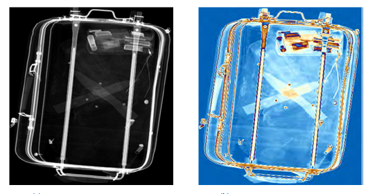
Figure 21. (a) The original grayscale image (b) the color-coded output, (c) the actual low-density threat (glass knife) concealed in the luggage

6. Evaluation

A comparison between color-coded images and grayscale-enhanced images is carried out to find out which people prefer. Three color coding methods and three grayscale methods were chosen for evaluation. Ten test images with low-density threats from our database are chosen for this survey. The steps involved are discussed in the following sections.

6.1 Procedure

The experiment was presented with the original gray scale image for comparison with the color-coded versions. The survey was carried out online and about thirty-five people took part in his survey. The survey was split into two portions, with five images in each survey. Three color-coding methods were evaluated with three grayscale-enhanced images. Cosine map, HSV method and rainbow map were chosen for color with the intensity stretched grayscale, negative and the histogram-equalized image. Each method is followed by three questions and finally the overall preference among the six presented method was noted. The survey was posted at http://web.utk.edu/~kkase/survey/.

Figure 22. Screen shot from the online survey showing the images followed by the Questions

6.2 Measures

Preference between grayscale and color-coded methods is to be measured. The primary dependent measure will be the ability to find the threat. Different factors considered in this study are:

Ability to detect threat

Are people able to detect threat?

Visual appeal

How pleasant / helpful the method is?

Time consumption

How long did it take to identify threat?

Overall preference

§ The visually best among the given methods

All the responses were tabulated in a excel file in the following format: the responses were tabulated in a excel file in the following format:

Table 1. Tabulated responses for each image

6.3 Survey results

The results showed that color-coding was significantly more effective than the no-coding (grayscale) images. Among the color-coding schemes, the rating was very close with HSV as most preferred followed by cosine and rainbow maps. The response plots (1,2,3,4) are shown below.

Each question is rated in a 1-10 scale with 10 the highest rating. For the over all preference the choices are among the six different display schemes, three of them were color and the rest based on grayscale. The responses were noted and the corresponding plot is shown in plot 1. Eighty-six percent (86%) of the total one hundred thirty two (132) responses, rated color as their preference.

Similarly, the responses for detect-ability, visual appeal and time taken to detect threat were noted and the plots are as shown below.

7. Conclusion

From the survey results, color has been shown superior to grayscale for effective information processing time and for memory performance. The ability to detect and identify details from the image is inherently increased by using color. Among the different coloring schemes the HSV scheme that was developed based on the color survey result was ranked highest by the greatest number of people. However, the other color maps were ranked very close to the HSV map. The cosine color map results were impressive. The difficulty with the HSV map is to set or pick the threshold. This can be solved by establishing an auto thresholding algorithm. The cosine color map produced very continuous and smooth results when compared to the other maps.

In addition, color-coding already enhanced images may produce better results. Currently color-coding is applied directly to the intensity stretched image. The survey was carried out with relatively few people. In the future, this study should be completed with more people to acquire statistically significant results. Also, the images should be presented in a pseudo random fashion to avoid the influence of other images in detecting the threat. False positives should be evaluated by introducing images without any threat. For more reliable results this survey should also be carried out with airport screeners.

Color should be used sparingly, consistently, and with clarity to aid in the formation of efficient mental models. Finally, use of the techniques and guidelines developed by Murch, Marcus and others. These rules, which were established from research, describe how colors fit together effectively.

Graphics:

MATLAB is an interactive environment in which you can program as well as visualize your computations. It includes a set of high-level graphical functions for:

§ Line plots (plot, plot3, polar)

§ Bar graphs (bar, barh, bar3, bar3h, hist, rose, pie, pie3)

§ Surface plots (surf, surfc)

§ Mesh plots (mesh, meshc, meshgrid)

§ Contour plots(contour, contourc, contourf)

§ Animation (moviein, movie)

MATLAB also provides for low-level control in the event that the user wishes to have better control of the graphical output.

In addition, MATLAB also provides a Graphical User Interface (GUI) toolbox called Guide for the creation of push buttons, text boxes, etc. for more user-friendly input to your m-files.

Using GUIDE Templates

GUIDE provides several templates, which are simple examples that you can modify to create your own GUIs. The templates are fully functional GUIs: their callbacks are already programmed. You can view the code for these callbacks to see how they work, and then modify the callbacks for your own purposes.

You can access the templates in two ways:

Start GUIDE by entering guide at the MATLAB prompt.
If GUIDE is already open, select New from the File menu in the Layout Editor.

Starting GUIDE displays the GUIDE Quick Start dialog as shown in the following figure.

The Quick Start dialog gives you two options:

Select the Open Existing GUI tab and open a GUI that you have already created.
Select the Create New GUI tab and open one of the templates.

The preceding figure shows the Quick Start dialog with the Create New GUI tab selected. Selecting a template in the left pane displays a preview in the right pane. Clicking OK opens the GUI template in the Layout Editor. If you select Save on startup as and type in name in the field to the right, GUIDE saves the GUI before opening it in the Layout Editor. If you choose not to save the GUI at this point, GUIDE prompts you to save it the first time you run the GUI.

GUIDE provides four templates, which are described in the following sections:

Blank GUI
GUI with Uicontrols
GUI with Axes and Menu
Modal Question Dialog

To view the M-file for any of these templates, open the template in the Layout Editor and click the M-file Editor icon

on the toolbar.

Blank GUI

The blank GUI template displayed in the Layout Editor is shown in the following figure.

GUI with Axes and Menu

The GUI with axes and menu template is shown in the following figure.

When you run the GUI by clicking the Run icon

on the toolbar, the GUI displays a plot of five random numbers generated by the MATLAB rand(5) command, as shown in the following figure.

You can select other plots in the pop-up menu. Clicking the Update button displays the currently selected plot on the axes.

The GUI also has a File menu with three items:

Selecting Open displays a dialog from which you can open files on your computer.
Selecting Print executes the printdlg command, which opens the Print dialog:

o    printdlg(handles.figure1)

·         Note that handles.figure1 contains the current plot. Clicking Yes in the Print dialog prints the plot.

·         Selecting Close closes the GUI.

Creating graphical user interface:

Saving and Running a GUI

After writing the callbacks, you can run the GUI by selecting Run from the Tools menu or clicking the Run button on the GUIDE toolbar. If you have not saved the GUI recently, GUIDE displays the following dialog box.

If this happens, click Yes and then save the GUI files to a writable directory.

Note GUI FIG-files that are created or modified with MATLAB 7.0 or a later MATLAB version, are not automatically compatible with Version 6.5 and earlier versions. To make a FIG-file, which is a kind of MAT-file, backward compatible, you must check the MAT-file Ensure backward compatibility (-v6) preference in the Preferences dialog box under General -> MAT-Files.

Note that uibuttongoups and uipanels are introduced in MATLAB 7.0, and you should not use them in GUIs that you expect to run in earlier MATLAB versions.

If the directory where you save the GUI is not on the MATLAB path, GUIDE opens the following dialog, giving you the option of changing the current working directory to the directory containing the GUI files, or adding that directory to the MATLAB path.

Click OK to change the current working directory. GUIDE then opens the GUI as shown in the following figure.

Note The name of the FIG-file saved by the Layout Editor and the generated M-file must match. See Renaming GUI Files if you want to rename files after first activating the GUI.

Next, select membrane in the pop-up menu and click the Contour push button. The GUI should look like the following figure.

Try experimenting with this GUI by adding another data set in the opening function, and a push button that displays a plot of the data set. Make sure to add the name of the new data set to the pop-up menu as well.

For more examples of creating GUIs with GUIDE, see the following sections:

"GUI Applications
Using GUIDE Templates

M-Files:

An M-File, with extension .m, that contains the code that controls the GUI, including the callbacks for its components.

Code

1. MATLAB coding for HSV color-map

clear all;

[fname,pname]=uigetfile('*.jpg','Browse to....');

im=imread(fname);

% deletes the xtra black space around the image

%img = trimimage(img);

subplot(2,2,1);

imshow(im);

img=rgb2gray(im);

subplot(2,2,2);

imshow(img);

% intensity adjustment

mmax=max(max(img));

mmax=double(mmax)/255 ;

img = imadjust(img,[0 mmax],[0 1]);

subplot(2,2,3);

imshow(img);

% size of the image

[m,n] = size(img);

newImg = zeros(m,n,3); %rgb format

% Setting the threshold

threshold = [0 1000 10000 35000 65535]/255;

% Fix the selected Hue

hue = [0.7, 0.4179, 1, 0.0850];

% ex % orange, green, blue (0.0850, 0.4179, 0.58170)

for i=1:length(threshold)-1

grayImg = imadjust(img,[threshold(i) threshold(i+1)]/255, []);

h = zeros(m,n);

s = h;

v = h;

[I,J] = find((img>=threshold(i)) & (img<threshold(i+1)));

ind = sub2ind([m,n],I,J);

h(ind) = hue(i);

s = 1;

v(ind) = ((double(grayImg(ind))/65535)/2) + 0.1; % 0.1 is added as an offset

vmax=max(max(v));

v = imadjust(v,[0 vmax],[0 1]);

hsvImg = zeros(m,n,3);

hsvImg(:,:,1) = h;

hsvImg(:,:,2) = s;

hsvImg(:,:,3) = v;

rgbImg = hsv2rgb(hsvImg); % convert HSV to RGB

newImg = imadd(newImg,rgbImg);

end

subplot(2,2,4);

imshow(newImg);

title('final image');

2. MATLAB coding for Cosine color-map

%**************************************************************

% This program uses a cosine function for transforming input gray

% image (.tif format) into a RGB image. f and p are the phase and

% frequency. These values can be varied and different color-coding

% schemes are obtained accordingly.

%**************************************************************

clear all

% getting the image from the file

[fname,pname]=uigetfile('*.jpg','Browse to....');

im=imread(fname);

% deletes the xtra black space around the image

%img = trimimage(img);

subplot(2,2,1);

imshow(im);

img=rgb2gray(im);

subplot(2,2,2);

imshow(img);

% Intensity adjustment

mmax=max(max(img));

mmax=double(mmax)/255 ;

img1 = imadjust(img,[0 mmax],[0 1]);

f=.9; % Frequency

p=.2; % Phase

[r,c]=size(img1);

subplot(2,2,3);

imshow(img1);

z=double(img1(1:r,1:c))/255;

img2(1:r,1:c,1) = (abs(cos(2*pi*f*z)));

img2(1:r,1:c,2) = abs(cos(2*pi*f*z+.5*p));

img2(1:r,1:c,3) = abs(cos(2*pi*f*z+p));

subplot(2,2,4);

imshow(img2);

3. MATLAB coding for rainbow (LUT)

%This program uses cosine function to produce rainbow color coding.

clear all

% getting the image from the file

[fname,pname]=uigetfile('*.jpg','Browse to....');

im=imread(fname);

figure,imshow(im);

img=rgb2gry(im);

figure,imshow(img);

% deletes the xtra black space around the image

% img = trimimage(img);

% intensity adjustment

mmax=max(max(img));

mmax=double(mmax)/255 ;

img1 = imadjust(img,[0 mmax],[0 1]);

figure,imshow(img1);

% histogram of the image

% figure, imhist(img1,64)

[r,c]=size(img1);

% h = waitbar(0,'Processing...');

level=input('Enter the number of COLOR levels:');

for i=1:level

map(i,1)=(1+cos((4*pi*double(i))/(3*255)))/2;

map(i,2)=(1+cos((4*pi*double(i)/(3*255))-(2*pi/3)))/2;

map(i,3)=(1+cos((4*pi*double(i)/(3*255))-(4*pi/3)))/2;

end

figure,imshow(img1)

colormap(map)

M-File of Pseudo Coloring in GUI

function varargout = pseudogui(varargin)

% PSEUDOGUI M-file for pseudogui.fig

% PSEUDOGUI, by itself, creates a new PSEUDOGUI or raises the existing

% singleton*.

% H = PSEUDOGUI returns the handle to a new PSEUDOGUI or the handle to

% the existing singleton*.

% PSEUDOGUI('CALLBACK',hObject,eventData,handles,...) calls the local

% function named CALLBACK in PSEUDOGUI.M with the given input arguments.

% PSEUDOGUI('Property','Value',...) creates a new PSEUDOGUI or raises the

% existing singleton*. Starting from the left, property value pairs are

% applied to the GUI before pseudogui_OpeningFunction gets called. An

% unrecognized property name or invalid value makes property application

% stop. All inputs are passed to pseudogui_OpeningFcn via varargin.

% *See GUI Options on GUIDE's Tools menu. Choose "GUI allows only one

% instance to run (singleton)".

% See also: GUIDE, GUIDATA, GUIHANDLES

% Edit the above text to modify the response to help pseudogui

% Last Modified by GUIDE v2.5 08-Feb-2008 15:44:56

% Begin initialization code - DO NOT EDIT

gui_Singleton = 1;

gui_State = struct('gui_Name', mfilename, ...

'gui_Singleton', gui_Singleton, ...

'gui_OpeningFcn', @pseudogui_OpeningFcn, ...

'gui_OutputFcn', @pseudogui_OutputFcn, ...

'gui_LayoutFcn', [] , ...

'gui_Callback', []);

if nargin & isstr(varargin{1})

gui_State.gui_Callback = str2func(varargin{1});

end

if nargout

[varargout{1:nargout}] = gui_mainfcn(gui_State, varargin{:});

else

gui_mainfcn(gui_State, varargin{:});

end

% End initialization code - DO NOT EDIT

% --- Executes just before pseudogui is made visible.

function pseudogui_OpeningFcn(hObject, eventdata, handles, varargin)

% This function has no output args, see OutputFcn.

% hObject handle to figure

% eventdata reserved - to be defined in a future version of MATLAB

% handles structure with handles and user data (see GUIDATA)

% varargin command line arguments to pseudogui (see VARARGIN)

axes(handles.axes1); axis off;

axes(handles.axes2); axis off;

axes(handles.axes3); axis off;

axes(handles.axes4); axis off;

axes(handles.axes5); axis off;

% HSV Method Initialization

handles.hue1 = 0.7;

handles.hue2 = 0.4179;

handles.hue3 = 1;

handles.hue4 = 0.0850;

%Cosine Method Initialization

handles.freq = 0.9;

handles.ph = 0.2;

% Choose default command line output for pseudogui

handles.output = hObject;

% Update handles structure

guidata(hObject, handles);

% UIWAIT makes pseudogui wait for user response (see UIRESUME)

% uiwait(handles.figure1);

% --- Outputs from this function are returned to the command line.

function varargout = pseudogui_OutputFcn(hObject, eventdata, handles)

% varargout cell array for returning output args (see VARARGOUT);

% hObject handle to figure

% eventdata reserved - to be defined in a future version of MATLAB

% handles structure with handles and user data (see GUIDATA)

% Get default command line output from handles structure

varargout{1} = handles.output;

% --- Executes on button press in pushbutton1.

function pushbutton1_Callback(hObject, eventdata, handles)

% hObject handle to pushbutton1 (see GCBO)

% eventdata reserved - to be defined in a future version of MATLAB

% handles structure with handles and user data (see GUIDATA)

[handles.fname, handles.pname]=uigetfile('*.jpg','Browse to....');

handles.img=imread([handles.pname handles.fname]);

handles.img = rgb2gray(handles.img);

mmax=max(max(handles.img));

mmax=double(mmax)/256;

handles.img = imadjust(handles.img,[0 mmax],[0 1]);

axes(handles.axes1);

imshow(handles.img); title('Input Image');

axes(handles.axes2);

imshow(imcomplement(handles.img)); title('Image Negative');

guidata(hObject, handles);

% --- Executes on button press in hsv.

function hsv_Callback(hObject, eventdata, handles)

% hObject handle to hsv (see GCBO)

% eventdata reserved - to be defined in a future version of MATLAB

% handles structure with handles and user data (see GUIDATA)

% size of the image

[m,n] = size(handles.img);

newImg = zeros(m,n,3); %rgb format

% Setting the threshold

threshold = [0 1000 10000 35000 65535]/256;

% Fix the selected Hue

%hue = [0.7, 0.4179, 1, 0.0850];

hue = [handles.hue1, handles.hue2, handles.hue3, handles.hue4];

% ex % orange, green, blue (0.0850, 0.4179, 0.58170)

for i=1:length(threshold)-1

grayImg = imadjust(handles.img,[threshold(i) threshold(i+1)]/256, []);

h = zeros(m,n);

s = h;

v = h;

[I,J] = find((handles.img>=threshold(i)) & (handles.img<threshold(i+1)));

ind = sub2ind([m,n],I,J);

h(ind) = hue(i);

s = 1;

v(ind) = ((double(grayImg(ind))/65535)/2) + 0.1; % 0.1 is added as an offset

vmax=max(max(v));

v = imadjust(v,[0 vmax],[0 1]);

hsvImg = zeros(m,n,3);

hsvImg(:,:,1) = h;

hsvImg(:,:,2) = s;

hsvImg(:,:,3) = v;

rgbImg = hsv2rgb(hsvImg); % convert HSV to RGB

newImg = imadd(newImg,rgbImg);

end

axes(handles.axes3); imshow(newImg); title('Output Image');

% --- Executes on button press in cosine.

function cosine_Callback(hObject, eventdata, handles)

% hObject handle to cosine (see GCBO)

% eventdata reserved - to be defined in a future version of MATLAB

% handles structure with handles and user data (see GUIDATA)

%figure, imshow(img)

% Intensity adjustment

mmax=max(max(handles.img));

mmax=double(mmax)/256 ;

img1 = imadjust(handles.img,[0 mmax],[0 1]);

f=handles.freq; % Frequency

p=handles.ph; % Phase

[r,c]=size(img1);

z=double(img1(1:r,1:c))/256;

img2(1:r,1:c,1) = (abs(cos(2*pi*f*z)));

img2(1:r,1:c,2) = abs(cos(2*pi*f*z+.5*p));

img2(1:r,1:c,3) = abs(cos(2*pi*f*z+p));

axes(handles.axes4); imshow(img2); title('Output Image');

% --- Executes on button press in rainbow.

function rainbow_Callback(hObject, eventdata, handles)

% hObject handle to rainbow (see GCBO)

% eventdata reserved - to be defined in a future version of MATLAB

% handles structure with handles and user data (see GUIDATA)

% histogram of the image

% figure, imhist(img1,64)

[r,c]=size(handles.img);

% h = waitbar(0,'Processing...');

%level=input('Enter the number of COLOR levels:');

%level = 200;

level = str2double(inputdlg('Enter the Number of Color Levels(100-255)'));

for i=1:level

map(i,1)=(1+cos((4*pi*double(i))/(3*255)))/2;

map(i,2)=(1+cos((4*pi*double(i)/(3*255))-(2*pi/3)))/2;

map(i,3)=(1+cos((4*pi*double(i)/(3*255))-(4*pi/3)))/2;

end

temp = ind2rgb(handles.img, map);

axes(handles.axes5); imshow(temp); title('Output Image');

% --- Executes during object creation, after setting all properties.

function hue1_CreateFcn(hObject, eventdata, handles)

% hObject handle to hue1 (see GCBO)

% eventdata reserved - to be defined in a future version of MATLAB

% handles empty - handles not created until after all CreateFcns called

% Hint: slider controls usually have a light gray background, change

% 'usewhitebg' to 0 to use default. See ISPC and COMPUTER.

usewhitebg = 1;

if usewhitebg

set(hObject,'BackgroundColor',[.9 .9 .9]);

else

set(hObject,'BackgroundColor',get(0,'defaultUicontrolBackgroundColor'));

end

% --- Executes on slider movement.

function hue1_Callback(hObject, eventdata, handles)

% hObject handle to hue1 (see GCBO)

% eventdata reserved - to be defined in a future version of MATLAB

% handles structure with handles and user data (see GUIDATA)

% Hints: get(hObject,'Value') returns position of slider

% get(hObject,'Min') and get(hObject,'Max') to determine range of slider

handles.hue1 = get(hObject,'Value');

guidata(hObject, handles);

% --- Executes during object creation, after setting all properties.

function hue2_CreateFcn(hObject, eventdata, handles)

% hObject handle to hue2 (see GCBO)

% eventdata reserved - to be defined in a future version of MATLAB

% handles empty - handles not created until after all CreateFcns called

% Hint: slider controls usually have a light gray background, change

% 'usewhitebg' to 0 to use default. See ISPC and COMPUTER.

usewhitebg = 1;

if usewhitebg

set(hObject,'BackgroundColor',[.9 .9 .9]);

else

set(hObject,'BackgroundColor',get(0,'defaultUicontrolBackgroundColor'));

end

% --- Executes on slider movement.

function hue2_Callback(hObject, eventdata, handles)

% hObject handle to hue2 (see GCBO)

% eventdata reserved - to be defined in a future version of MATLAB

% handles structure with handles and user data (see GUIDATA)

% Hints: get(hObject,'Value') returns position of slider

% get(hObject,'Min') and get(hObject,'Max') to determine range of slider

handles.hue2 = get(hObject,'Value');

guidata(hObject, handles);

% --- Executes during object creation, after setting all properties.

function hue3_CreateFcn(hObject, eventdata, handles)

% hObject handle to hue3 (see GCBO)

% eventdata reserved - to be defined in a future version of MATLAB

% handles empty - handles not created until after all CreateFcns called

% Hint: slider controls usually have a light gray background, change

% 'usewhitebg' to 0 to use default. See ISPC and COMPUTER.

usewhitebg = 1;

if usewhitebg

set(hObject,'BackgroundColor',[.9 .9 .9]);

else

set(hObject,'BackgroundColor',get(0,'defaultUicontrolBackgroundColor'));

end

% --- Executes on slider movement.

function hue3_Callback(hObject, eventdata, handles)

% hObject handle to hue3 (see GCBO)

% eventdata reserved - to be defined in a future version of MATLAB

% handles structure with handles and user data (see GUIDATA)

% Hints: get(hObject,'Value') returns position of slider

% get(hObject,'Min') and get(hObject,'Max') to determine range of slider

handles.hue3 = get(hObject,'Value');

guidata(hObject, handles);

% --- Executes during object creation, after setting all properties.

function hue4_CreateFcn(hObject, eventdata, handles)

% hObject handle to hue4 (see GCBO)

% eventdata reserved - to be defined in a future version of MATLAB

% handles empty - handles not created until after all CreateFcns called

% Hint: slider controls usually have a light gray background, change

% 'usewhitebg' to 0 to use default. See ISPC and COMPUTER.

usewhitebg = 1;

if usewhitebg

set(hObject,'BackgroundColor',[.9 .9 .9]);

else

set(hObject,'BackgroundColor',get(0,'defaultUicontrolBackgroundColor'));

end

% --- Executes on slider movement.

function hue4_Callback(hObject, eventdata, handles)

% hObject handle to hue4 (see GCBO)

% eventdata reserved - to be defined in a future version of MATLAB

% handles structure with handles and user data (see GUIDATA)

% Hints: get(hObject,'Value') returns position of slider

% get(hObject,'Min') and get(hObject,'Max') to determine range of slider

handles.hue4 = get(hObject,'Value');

guidata(hObject, handles);

% --- Executes during object creation, after setting all properties.

function freq_CreateFcn(hObject, eventdata, handles)

% hObject handle to freq (see GCBO)

% eventdata reserved - to be defined in a future version of MATLAB

% handles empty - handles not created until after all CreateFcns called

% Hint: slider controls usually have a light gray background, change

% 'usewhitebg' to 0 to use default. See ISPC and COMPUTER.

usewhitebg = 1;

if usewhitebg

set(hObject,'BackgroundColor',[.9 .9 .9]);

else

set(hObject,'BackgroundColor',get(0,'defaultUicontrolBackgroundColor'));

end

% --- Executes on slider movement.

function freq_Callback(hObject, eventdata, handles)

% hObject handle to freq (see GCBO)

% eventdata reserved - to be defined in a future version of MATLAB

% handles structure with handles and user data (see GUIDATA)

% Hints: get(hObject,'Value') returns position of slider

% get(hObject,'Min') and get(hObject,'Max') to determine range of slider

handles.freq = get(hObject,'Value');

guidata(hObject, handles);

% --- Executes during object creation, after setting all properties.

function ph_CreateFcn(hObject, eventdata, handles)

% hObject handle to ph (see GCBO)

% eventdata reserved - to be defined in a future version of MATLAB

% handles empty - handles not created until after all CreateFcns called

% Hint: slider controls usually have a light gray background, change

% 'usewhitebg' to 0 to use default. See ISPC and COMPUTER.

usewhitebg = 1;

if usewhitebg

set(hObject,'BackgroundColor',[.9 .9 .9]);

else

set(hObject,'BackgroundColor',get(0,'defaultUicontrolBackgroundColor'));

end

% --- Executes on slider movement.

function ph_Callback(hObject, eventdata, handles)

% hObject handle to ph (see GCBO)

% eventdata reserved - to be defined in a future version of MATLAB

% handles structure with handles and user data (see GUIDATA)

% Hints: get(hObject,'Value') returns position of slider

% get(hObject,'Min') and get(hObject,'Max') to determine range of slider

handles.ph = get(hObject,'Value');

guidata(hObject, handles);

CONCLUSION:

The GUI for performing above operations with out giving inputs is as shown in the figure below:

The input to which the transformations are to be applied is selected from the files by pressing the select input image pushbutton.

COSINE COLORMAP :

Mathematical functions are utilized to perform the required transformation from gray scale to color. This is performed in the RGB color space. The idea is to perform three independent transformations of the gray level of any input pixel. The three results are combined together as red, green and blue channel to produce a color-coded image.

RAINBOW COLORMAP:

This color map (LUT) is applied to the original grayscale image to obtain pseudo colored output image.

HSV COLORMAP:

The application of image threshold techniques for the selective visualization of certain gray-level brackets, leads to isolated and enhanced threat representations.The basic procedure is as follows:

(1). The thresholds are set

(2). The number of colors to be used is defined

(3). The hues to be used are defined

(4). In the HSV space the hues are set for each threshold, the saturation is set to one and the value is set to the intensity value of the pixel

(5). Step 4 is repeated for all the thresholds

(6). Then the HSV image is transformed to RGB space for display

The output image thus obtained after applying all the above color transforms is as shown below:

APPLICATION:

Pseudocolour Image Processing in Digital Mammography:

Mammography is not a simple radiological technique alone, which is used to image breast tissues as it was known for the past two decades till 1996. Mammography is the leading method for breast imaging today. Pseudo coloring is applied for the 2D images taken in two plain film (X-ray) mammography at an angle 450 / 900 between them and the details are collected in digital form in a computer for segmentation and reconstruction. In this diagnostic process, Pseudo coloring plays a vital role in the detection of presumptive breast cancer or occult carcinoma.